Estimating energy expenditure from workout data
A fitness application needs to turn information such as workout duration, heart rate, and user characteristics into a useful estimate of energy expenditure. This project investigates that prediction problem using recorded Calories_Burned as the target.
I carried the study from CSV intake in KNIME through feature engineering, model fitting, and evaluation in SAS Visual Analytics / Viya. The central challenge was building a trustworthy comparison: repeated records could inflate validation performance, plausible extreme workouts needed careful treatment, and the models needed to be assessed beyond a single score.
1. Auditing the records before modeling
Removing duplicates before the split
The raw gym_members_exercise_tracking.csv contained 4,865 rows, but only 973 distinct observations, each repeated five times. I removed the duplicates before creating training and validation partitions. Otherwise, the same workout could appear in both partitions, making the model look successful at predicting data it had effectively already seen.
This decision determines whether the later validation comparison is meaningful. More rows would have made the input look larger without adding new information.
Checking completeness and internal consistency
The Statistics node showed no missing values across the original 15 variables. I also recalculated BMI from weight divided by height squared and compared it with the supplied values. Differences were below 0.0050, consistent with the source rounding BMI to two decimal places.
That audit checks a relationship between fields rather than treating every populated value as automatically reliable. It also avoids replacing a consistent supplied feature unnecessarily.
Investigating outliers in context
I used a 1.5 × IQR rule to flag unusual numeric values, including calorie expenditure above approximately 1,613 kcal and weight above 127.8 kg. The high-calorie observations inspected in the report involved experienced participants, average heart rates above 160 BPM, and sessions around two hours long.
I retained plausible high-performance observations instead of deleting every flagged value. For a calorie estimator, removing legitimate intense workouts would narrow the behavior represented in the training data. The flag is a reason to investigate; the surrounding workout information guides the treatment.
The workflow on the project cover is repeated below. It shows how intake and deduplication feed the audit, calculated features, and final export.
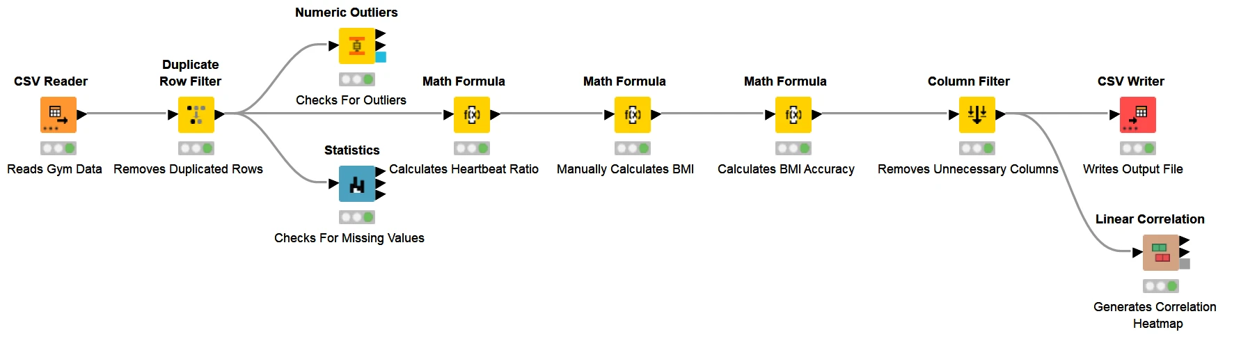
The workflow carries CSV intake through deduplication, outlier and completeness checks, BMI and heart-rate calculations, correlation analysis, and export. Removing repeated observations before the split protects the later model comparison.
View full-size figure2. Creating features and exploring relationships
Expressing heart rate relative to the participant
Average BPM describes the session, but resting and maximum heart rate provide personal context. I engineered a heart-rate intensity ratio using heart-rate reserve:
HR_Intensity_Ratio = (Avg_BPM − Resting_BPM)
                    / (Max_BPM − Resting_BPM)
This gives the model a relative-exertion feature alongside the original measurements. It demonstrates how domain knowledge can inform a calculated input; whether that input improves prediction still needs to be assessed in the modeling stage.
Using exploration to guide the model comparison
The correlation analysis showed a strong association between session duration and recorded calories (r ≈ 0.908). Experience level (0.694), workout frequency (0.576), fat percentage (−0.598), and average BPM (0.340) offered additional relationships to investigate.
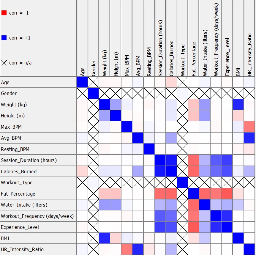
Duration has the strongest linear association with recorded calories. The matrix also exposes relationships among inputs, helping distinguish exploratory associations from the importance rankings produced by fitted models.
View full-size figureThese patterns helped me understand the inputs before fitting models. Correlation describes a linear association; it does not establish what causes calorie expenditure or guarantee a feature’s value once other predictors are included.
I exported gym_members_cleaned.csv with 973 rows and 16 columns, giving SAS a defined input table with the audited records and engineered intensity feature.
3. Fitting models and reading their diagnostics
I used a common simple random 70/30 partition: 681 training observations and 292 validation observations. Comparing the models on the same held-out records makes their errors directly comparable.
Linear regression: establishing a useful baseline
The stepwise regression used the Schwarz Bayesian Criterion (SBC) and retained session duration, average BPM, age, and gender. It provides a relatively simple reference for deciding whether the added complexity of tree ensembles is worthwhile.
The residual plot shows curvature rather than an evenly scattered pattern around zero. Reading that diagnostic helps identify structure the linear fit has not captured, even when its overall error is competitive.
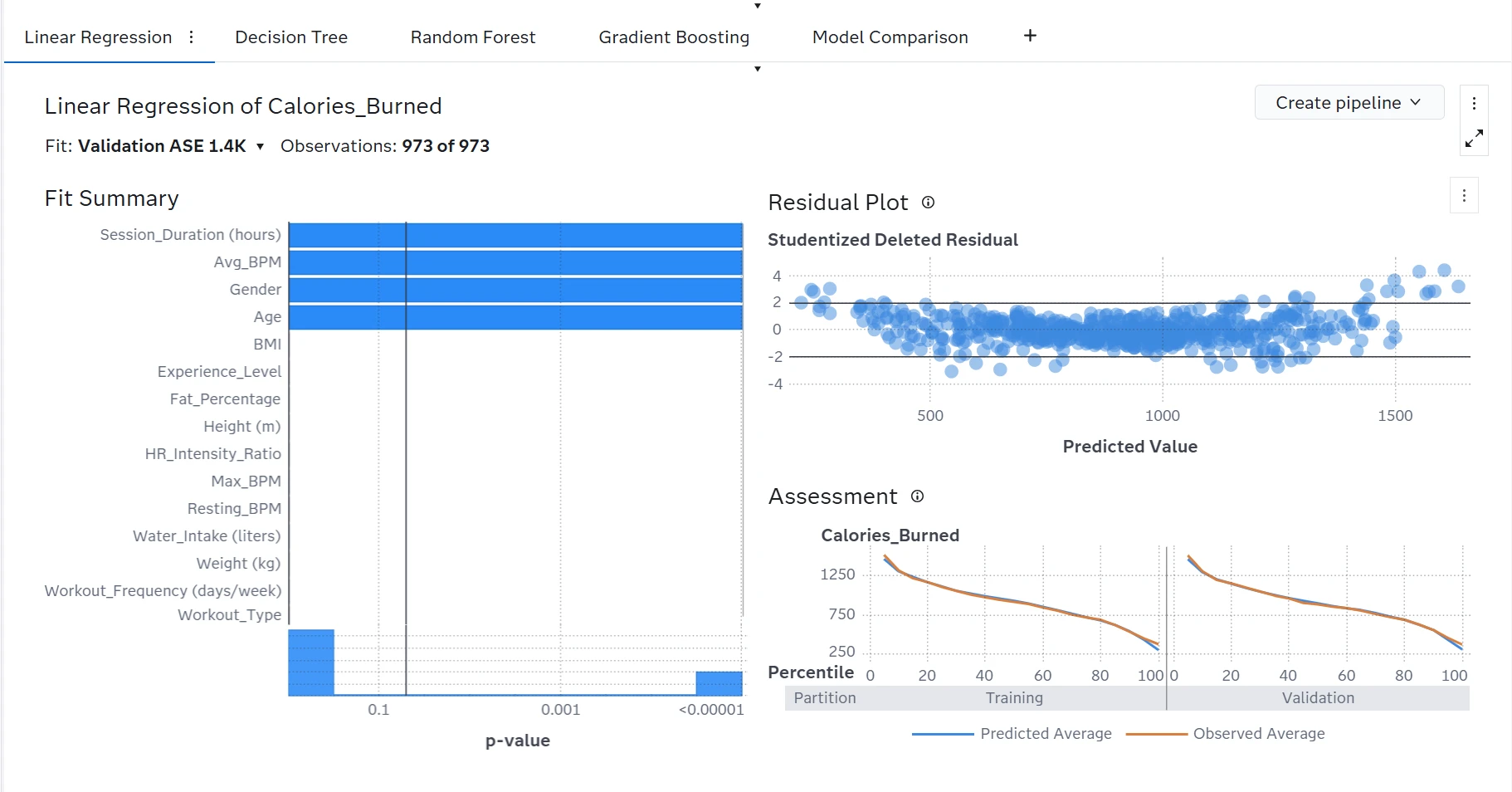
The baseline retains duration, average BPM, age, and gender. Curvature in the residuals reveals structure the linear fit misses, despite its competitive validation error.
View full-size figureDecision tree: making the prediction rules visible
I configured a binary tree with a maximum of five levels and a minimum leaf size of ten, using validation average squared error for pruning. Its first split is at 1.25 hours of session duration; later branches use average BPM and experience level.
The tree makes the segmentation easy to inspect. Its stepped predictions also reveal a limitation: workouts within a leaf receive the same predicted value, which can make a continuous target such as calories difficult to estimate precisely.
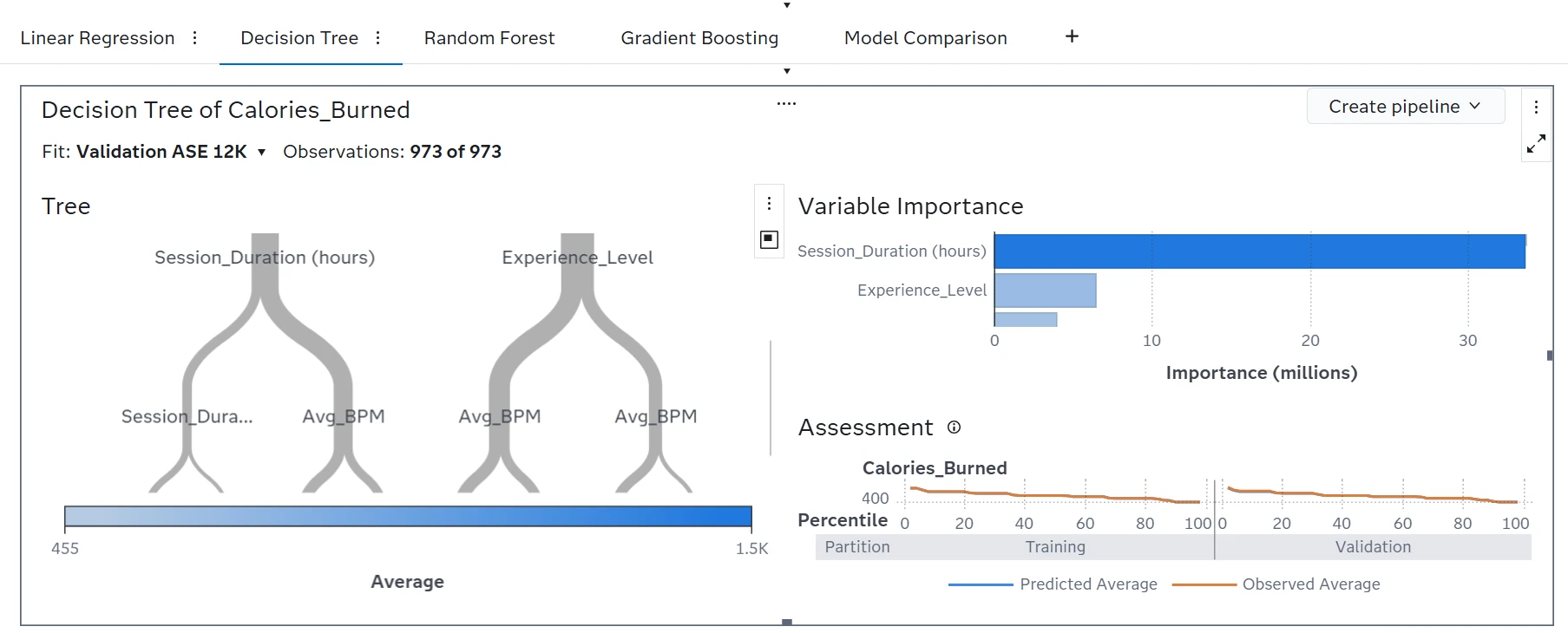
The tree segments workouts using duration, heart rate, and experience. Its constant predictions within leaves make the rules readable while limiting the precision of the continuous calorie estimate.
View full-size figureRandom forest: checking what the ensemble adds
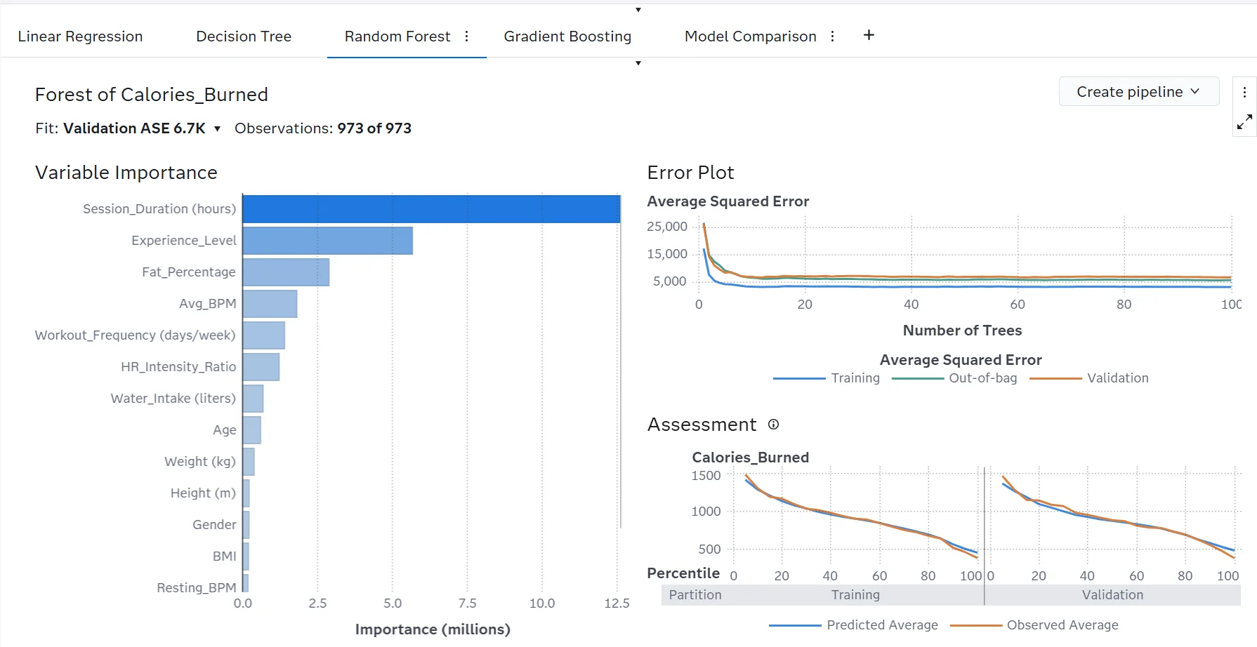
The forest used 100 trees, an in-bag sampling proportion of 0.6, five candidate predictors per split, and a maximum of ten levels. Its error curve falls and then levels off, showing how performance changes as trees are added.
Duration, experience, fat percentage, and average BPM feature prominently in its importance ranking. The diagnostic view lets me inspect both the model’s learning behavior and which inputs it uses, before comparing its validation error with the simpler alternatives.
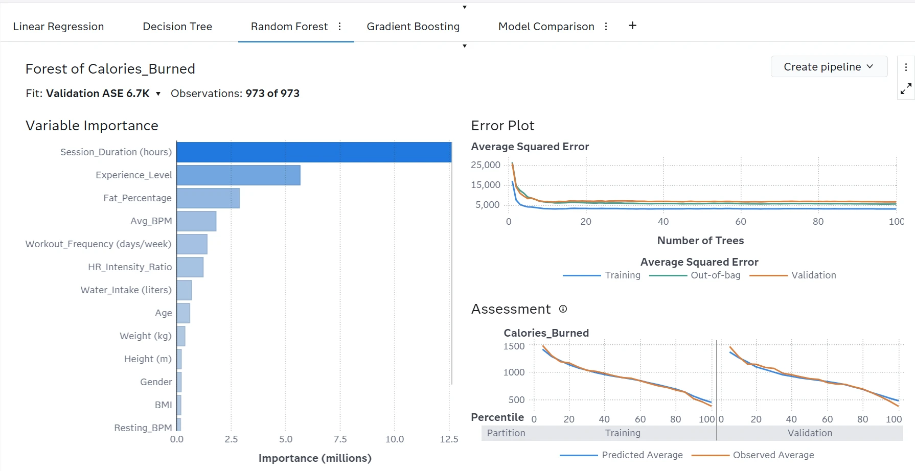
The error curve decreases and then plateaus. Duration leads the importance ranking, with experience, fat percentage, and average BPM also prominent; validation comparison determines whether the ensemble improves on the baseline.
View full-size figureGradient boosting: inspecting the strongest candidate
The boosting configuration used 100 trees, a 0.1 learning rate, 0.8 subsampling, and a maximum of four levels. Its page combines variable importance, training and validation error over iterations, and predicted versus observed averages.
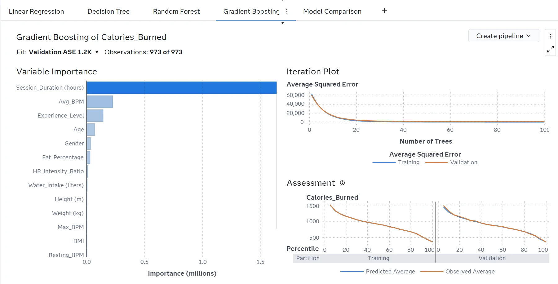
The selected candidate combines duration-led feature importance with iteration and assessment plots. Reading training and validation behavior together helps explain the result and keeps the generalization gap visible.
View full-size figureSession duration leads the importance ranking, followed by average BPM. The iteration plot helps assess whether improvements on training data carry through to validation. Looking at those views together gives a fuller explanation of the candidate’s behavior than simply naming it the winner.
4. Comparing prediction error in a meaningful unit
The SAS comparison table reports average squared error (ASE). Taking its square root expresses the result in kilocalories, the same unit as the prediction target:
| Model | Validation ASE | Validation RMSE |
|---|---|---|
| Linear regression | 1,362.5646 | 36.91 kcal |
| Decision tree | 11,644.4801 | 107.91 kcal |
| Random forest | 6,703.8423 | 81.88 kcal |
| Gradient boosting | 1,225.0708 | 35.00 kcal |
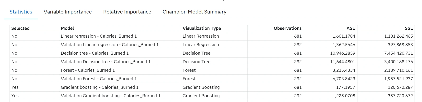
All four models use 681 training and 292 validation observations. Gradient boosting has the lowest validation ASE (1,225.0708, about 35 kcal RMSE), with linear regression close behind.
View full-size figureGradient boosting had the lowest validation error, but linear regression was close. That is a useful model-selection finding: a more complex model needs to justify its added cost against a credible baseline. The single tree and forest performed worse with the configurations used in this study.
Boosting’s training ASE was 177.1957, substantially below its validation ASE. The gap keeps overfitting an open evaluation concern. The 292 observations were used for model selection, so a fresh test set would be needed to assess the selected model independently. 35 kcal RMSE summarizes this validation result; individual predictions can have larger errors.
5. Connecting the model to a practical use case
The report proposes calorie estimates in a fitness app, heart-rate telemetry as an input, and onboarding tailored to experience level. The prepared data and model comparison provide a basis for exploring those applications: they define the inputs, identify influential predictors, and quantify error in a unit a product team can interpret.
Before putting those estimates into a live service, I would evaluate fresh workouts, compare errors across participant and activity groups, and examine missing context such as nutrition and recovery. Predictor importance alone cannot support precise exercise prescriptions.
The completed study demonstrates the work behind a useful prediction: checking the data, constructing an input with domain context, diagnosing different model behaviors, and communicating a result with its evaluation conditions. The figures are extracted from my submitted report.