Preparing customer data that a business can use
The trading-company scenario began with four regional Excel files. The files represented the same business, but their customer records contained different name structures, placeholder numbers, inconsistent financial values, and invalid birth dates. Those problems had to be addressed before the data could support reporting or customer analysis.
I designed a KNIME pipeline that carries the records through integration, cleaning, identifier masking, transformation, and analysis. Each stage has a practical purpose: preserve the source context, handle errors without discarding the rest of a customer record, create useful reporting fields, and deliver an organized master table. The finished output is Cleaned_Data.xlsx, supported by a visible workflow that makes the preparation decisions inspectable.
1. Combining the regional sources
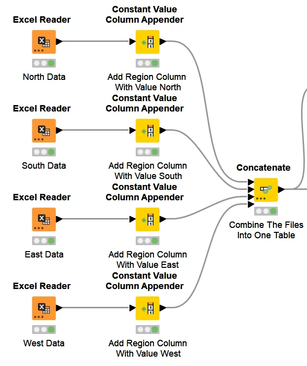
I created a separate Excel Reader branch for North, South, East, and West. Before combining them, I attached a Region column to every branch. This preserves where each record came from, so the same master table can later support both company-wide analysis and regional comparisons.
The Concatenate node stacks the records and creates new row IDs to avoid indexing conflicts. This intake stage is the workflow shown on the project cover and below: four regional inputs become one table without losing their regional context.
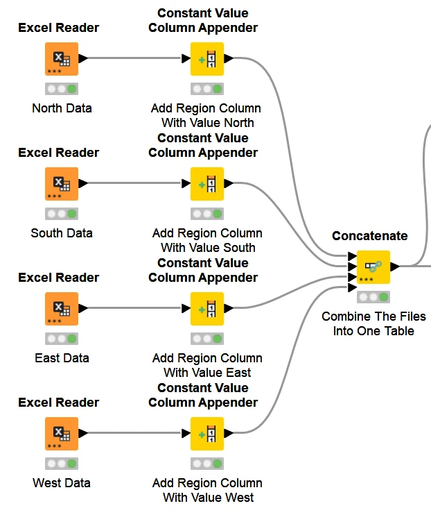
Each Excel Reader branch adds its regional label before concatenation. This preserves the source context needed by the later regional analysis, while new row IDs prevent indexing conflicts.
View full-size figure2. Cleaning values and reconciling schemas
I profiled the combined table with a Statistics node before deciding how to treat it. The initial profile exposed values such as 9999 in purchase and spending fields and an annual income recorded as 71. These entries would distort the financial summaries used later in the analysis.
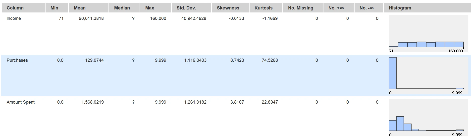
The initial profile reveals the financial anomalies that drive the cleaning rules. Inspecting ranges and distributions before treatment gives each transformation a reason.
View full-size figureI used a sequence of Rule Engine nodes to handle different errors explicitly:
- Purchases: turn the
9999placeholder into a missing value. - Amount spent: remove the placeholder and flag zero spending when purchases are recorded, while allowing zero spending for a customer with no purchases.
- Income: treat the placeholder and entries failing the workflow’s minimum-income rule as missing values.
- Credit-card use: convert
1and0into readableYesandNocategories.
The spending rule uses two columns together, showing how I translated a business relationship into a validation rule. The flag transformation makes the prepared data easier to interpret in reports.
For purchases, spending, and income, I filled missing entries with the column median. This keeps the customer’s other information available, and the median is less sensitive to extreme values than the mean. A second Statistics node checks the result: the captured profile shows no remaining missing values in these three financial fields.
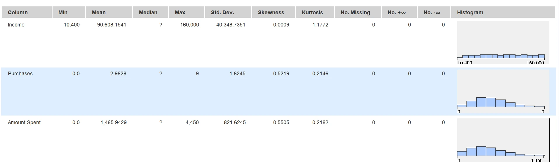
Profiling after rule-based treatment and median imputation checks income, purchases, and spending before they feed the business metrics. The captured profile shows no missing values in those three columns.
View full-size figureI then resolved a schema mismatch between branches. Some sources supplied one Name field; others supplied First Name and Last Name. String Manipulation combines the split names, Column Merger fills the primary field, and Column Filter removes the redundant columns. The result gives downstream reporting one consistent name field to work with.
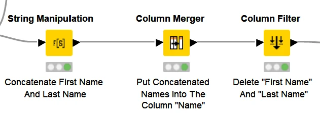
The regional files use different name structures. These three steps reconcile them into one field so downstream reporting can use a consistent schema.
View full-size figure3. Designing identifier masking
The customer table also contained an SSN field. I used String Manipulation to replace its first five digits with a fixed mask and retain the final four digits, producing the format XXX-XX-1234 for an example ending in 1234.
Writing the transformation explicitly gave me control over the output format and the portion retained. This is partial identifier masking; the table’s remaining personal fields still need appropriate handling when shared. The public figures show workflow steps and aggregate analysis.
4. Creating features and preparing the export
Deriving age and handling invalid dates
I used Date&Time Difference to calculate age from birth date and the workflow’s execution date. Profiling the new field revealed zero and negative ages caused by future-dated entries. I converted those invalid ages to missing values and applied median imputation, preserving the usable parts of the affected records.
This stage shows why derived features need their own checks: a date can be present and parse successfully while still producing an impossible age.
Creating demographic groups
I used Numeric Binner nodes to turn age and income into reporting categories. Age becomes Youth, Adult, or Senior using boundaries at 25 and 55. Income becomes Low, Medium, or High using boundaries at 50,000 and 100,000.
Those categories give the business a manageable way to compare customer groups. They also provide the fields used by the demographic charts in the final analysis.
Engineering average order value
I calculated each customer’s average order value from amount spent divided by purchases. The Math Formula includes an explicit zero-purchase case that returns zero, preventing undefined ratios from entering the output. A Number Rounder then formats the result to two decimal places.
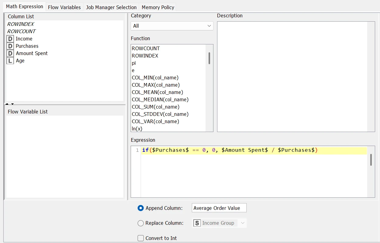
The formula creates a customer-level spending measure and handles zero purchases explicitly. This is the feature later averaged in the regional order-value chart.
View full-size figureThis metric adds a different view of purchasing behavior: a customer’s spending total and their average order size can tell different stories. Its later regional comparison depends on this calculation being defined consistently for every record.
Organizing the handoff
I reordered the columns into identity and location, demographic and financial information, and purchasing measures. I sorted records by region and descending spending, making each branch’s higher-spending customers easier to find during review.
The resulting Cleaned_Data.xlsx brings the source records, resolved schema, masked identifier, demographic groups, and spending features into one structured output. That is the central deliverable of the preparation workflow; the analysis below uses the fields built through these stages.
5. Analyzing the prepared customer data
Understanding the customer mix
The income-group chart shows 652 high-income, 548 medium-income, and 306 low-income customers. High income is the largest segment at about 43.3%. The chart makes the engineered categories useful for understanding the customer base and choosing groups for further investigation.
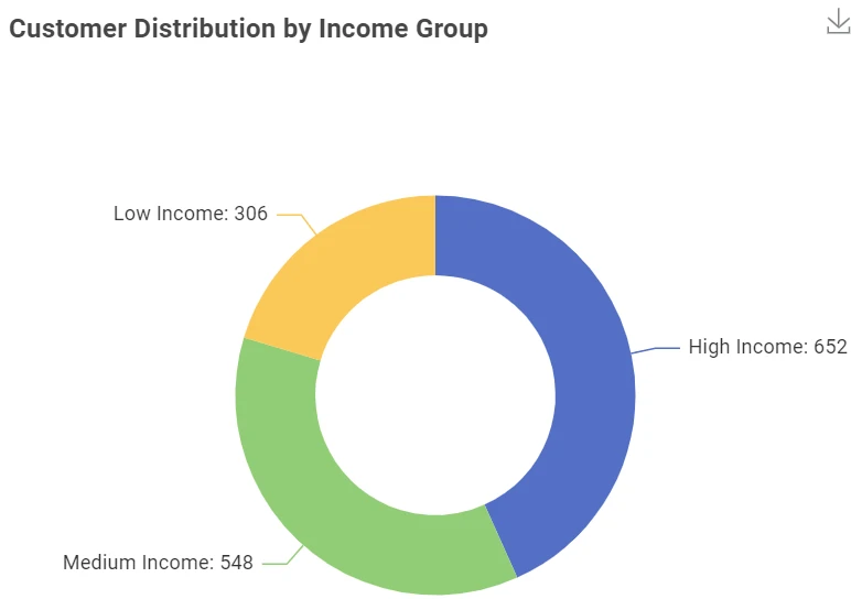
The Numeric Binner income groups become an interpretable customer profile: 652 high-income, 548 medium-income, and 306 low-income records.
View full-size figureComparing regional spending and order value
The regional chart compares average customer spending with the regional average of the customer-level order values calculated earlier. West leads average customer spending at 1,550.98, while South leads average order value at 482.29. Order values are fairly similar across the four regions.
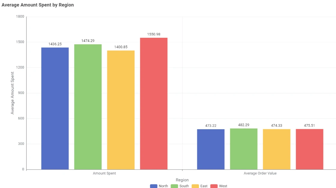
West leads average customer spending; South leads the regional average of customer-level order values. The distinction gives a retailer separate questions to investigate about purchase frequency and order size.
View full-size figureReading both measures together gives a more complete picture of regional purchasing behavior. It creates a useful next question about the contribution of purchase frequency and order size to customer spending. These are customer-level averages, so the chart answers a different question from a comparison of total regional revenue.
Checking the relationship between age and spending
I paired a scatter plot with Pearson correlation to examine whether spending increased with age. The coefficient is approximately 0.032, indicating very little linear association in the prepared dataset. The source profile also shows a median age of 74, so the concentration of older customers does not by itself explain differences in spending.
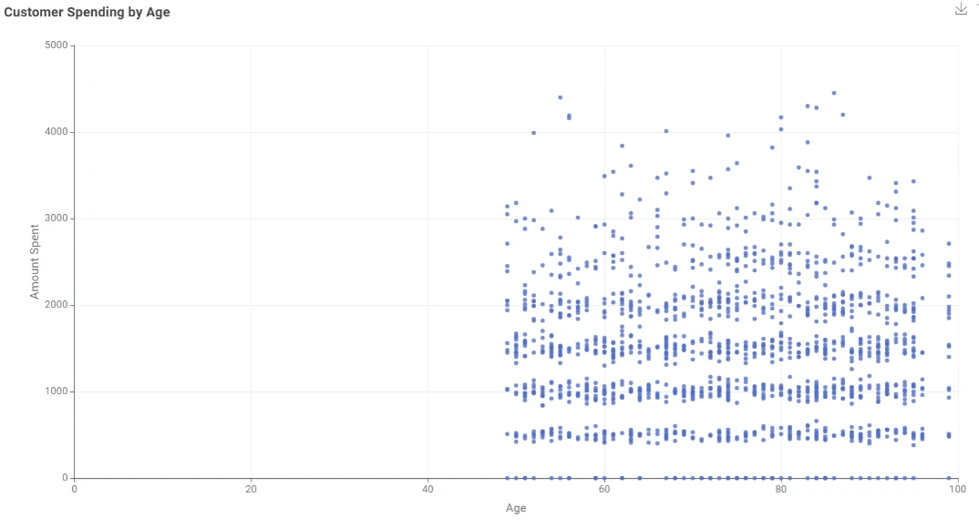
The scatter plot and Pearson correlation of approximately 0.032 give little support for using exact age as a linear spending signal in this dataset. Customer demographics and purchasing behavior answer different questions.
View full-size figureThe completed project connects data preparation to interpretation: I built the fields and consistent table needed to describe the customer base, compare regions, and examine a demographic assumption. The KNIME workflow and Excel output give the analysis a documented path back to its preparation decisions.