Making the mechanics of learning visible
NumPyGrad began with a question: could I build the machinery behind a neural network, then give people a way to explore what it actually does? I implemented reverse-mode automatic differentiation, trainable layers, optimizers, and checkpoint serialization in Python and NumPy. The core learning computations run without an external deep learning framework.
The Streamlit studio turns that engine into an interactive product. Its three main views are 2D Decision Boundaries, Autonomous Neural Pathfinding, and Handwritten Digit Recognition. The first view contains the training workspace, coordinate inference, computation trace, and model comparison. The journey below follows those interactions, then moves into the rover and drawing canvas.
This connects several parts of my engineering work: implementing the mathematics, evaluating models, making their behavior inspectable, and handling the input and presentation needed for a usable application. The six screenshots and rover recording on this page were supplied directly from my studio sessions.
1. Train a boundary and watch the model learn
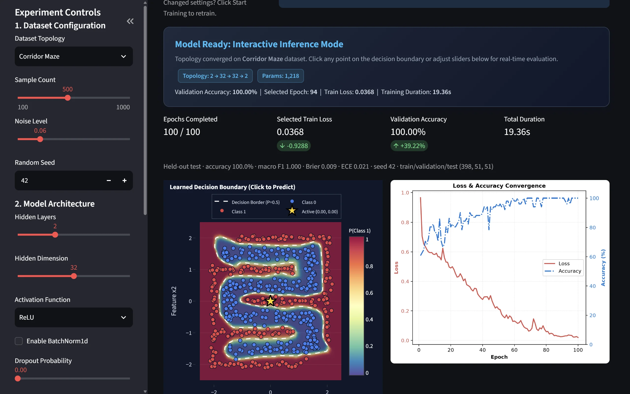
The first screen lets a visitor choose a dataset, adjust its sample count and noise, configure a network, and start training. The supplied example uses Corridor Maze, 500 points, and a 2 → 32 → 32 → 2 ReLU network. Batch normalization and dropout are available alongside optimizer and learning-rate controls.
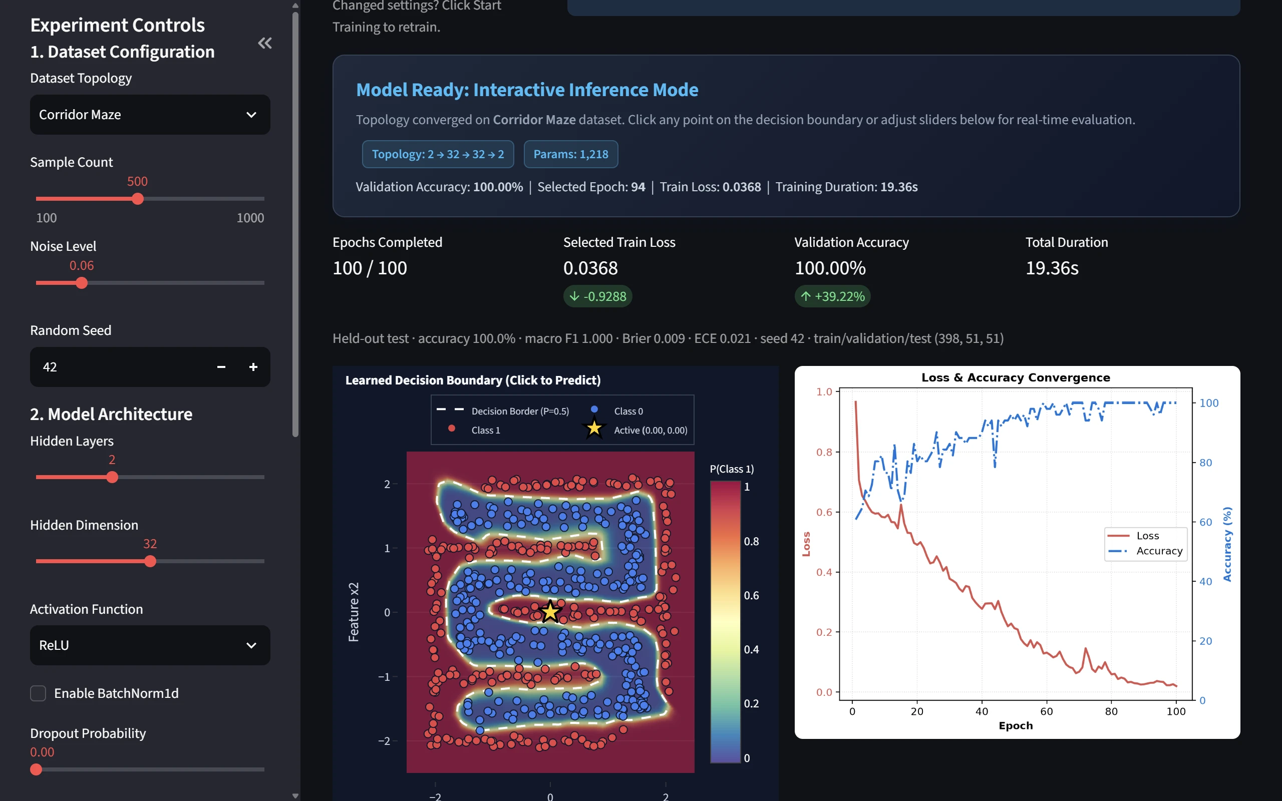
The project cover is this training workspace. The captured run selects epoch 94 by validation loss and reports 100% held-out accuracy, macro F1 1.000, Brier score 0.009, and ECE 0.021. These figures describe this synthetic-data session.
View full-size figureThe contour map shows where the model places its class boundary; the adjacent curves show training loss and validation accuracy as learning progresses. Connecting these views makes the result interpretable: the visitor can see whether lower loss produces a boundary that follows the winding corridor.
Evaluation is part of the training workflow
I split the observations into separate training, validation, and test partitions, approximately 80/10/10 in this configuration. For sufficiently populated corridor regions, the splitter stratifies by spatial region as well as class, helping keep narrow sections represented in evaluation. The captured run contains 398 training, 51 validation, and 51 test points.
The studio saves the state with the lowest validation loss and restores it before final test evaluation. In this session it selects epoch 94, rather than automatically using the last epoch. The capture reports 100% held-out accuracy, macro F1 1.000, Brier score 0.009, and expected calibration error 0.021. These are results for the captured synthetic dataset and split.
Reporting probability-quality measures alongside accuracy makes evaluation more useful: correct labels and well-behaved confidence scores are different properties. Checkpoint selection also separates the choice of model state from the held-out test assessment.
The engine behind Start Training
Each mini-batch passes through my Linear and activation layers, then the numerically stable CrossEntropyLoss. Calling loss.backward() traverses a dynamic computation graph in reverse topological order before SGD or AdamW updates the registered parameters.
forward → loss → backward → step- 01TensorData + gradient + parents
- 02Dynamic graphOperations record dependencies
- 03Backward passReverse topological traversal
- 04OptimizerUpdate registered parameters
The backward rules handle cases that matter in ordinary networks. Shared inputs accumulate contributions from every downstream branch. _unbroadcast sums batch contributions back into a bias tensor’s original shape. The Module hierarchy registers parameters and propagates training or evaluation mode through nested layers, giving dropout and batch normalization the appropriate behavior.
I checked those mechanics with centered finite-difference gradient comparisons and automated tests for graph ordering, branching, broadcasting, layers, and serialization. The gradient checker and test suite provide independent ways to inspect the implementation. This is the foundation that makes the studio’s training results meaningful.
2. Probe a prediction at a new coordinate
After training, a visitor can click the boundary plot, move the X1 and X2 sliders, or choose a preset such as the origin or a decision-border point. The active point appears on the map, while a prediction card and probability bars update alongside it. A logging control keeps selected test coordinates available for inspection.
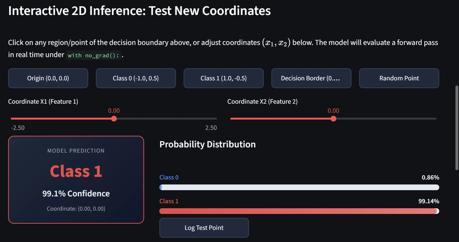
A point selected on the map, through sliders, or from a preset runs through the same trained model. At the origin in this capture, Class 1 has a 99.14% softmax score; test points can be logged for comparison.
View full-size figureAt (0, 0) in this session, the model predicts Class 1 with a 99.14% softmax score, versus 0.86% for Class 0. That score exposes how strongly the model favors its prediction; it is not a guarantee that a new point is classified correctly.
The same trained network evaluates a coordinate tensor of shape (1, 2) through its layers. I run the forward pass in evaluation mode inside no_grad(), which prevents autograd dependency recording and backward-graph retention during inference. This keeps prediction separate from training work and avoids building a graph that the interaction will never use.
The interaction gives the boundary plot a practical purpose: visitors can investigate confident regions and uncertain borders instead of only looking at a finished chart.
3. Open the computation trace and inspect the internals
The Engine Internals & Computation Trace drawer follows the active prediction into the implementation. It exposes intermediate layer outputs, the stable softmax calculation, parameter diagnostics, raw weights, and gradient-flow telemetry.
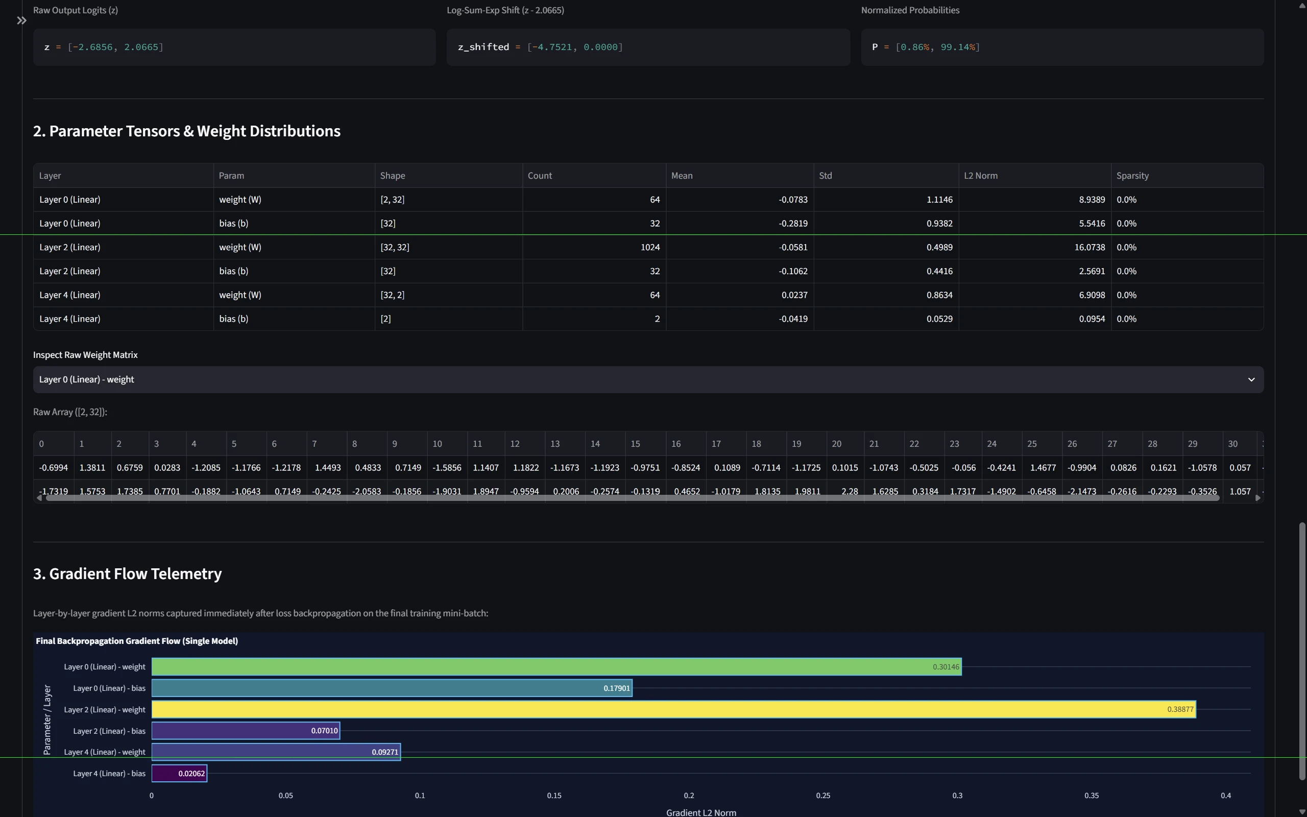
The drawer exposes the numerical calculation, registered parameter tensors, and gradient-flow telemetry. Gradient norms come from the final training mini-batch; the restored validation checkpoint supplies inference weights.
View full-size figureFollow the numerical calculation
The displayed logits are approximately [-2.6856, 2.0665]. Subtracting their maximum gives [-4.7521, 0] before exponentiation and normalization. This shift preserves the softmax result while avoiding overflow for large positive logits. The same numerical-stability principle underpins the engine’s log-sum-exp cross-entropy calculation.
Inspect what the model learned
The parameter table shows the layer shapes, means, standard deviations, L2 norms, and sparsity, with a selector for viewing the actual weight arrays. For this model, the weight matrices have shapes [2, 32], [32, 32], and [32, 2], accompanied by their bias tensors.
The gradient chart shows parameter-gradient norms recorded immediately after backpropagation on the final training mini-batch. Those values help investigate uneven or weak gradient flow across layers. They describe that training step; the inference weights come from the separately restored validation checkpoint.
Building these views required exposing useful state from the tensor and module APIs. The result is a debugging and teaching surface where a reader can connect a prediction to the numerical operations and parameters that produced it.
4. Compare model configurations on the same experiment
Switching to Model Capacity Comparison (A vs B) lets a visitor configure two models and train them together. Both use the same split and mini-batch sequence, then retain their own best-validation checkpoints. The screen compares boundaries, convergence curves, held-out diagnostics, and predictions for a shared coordinate.
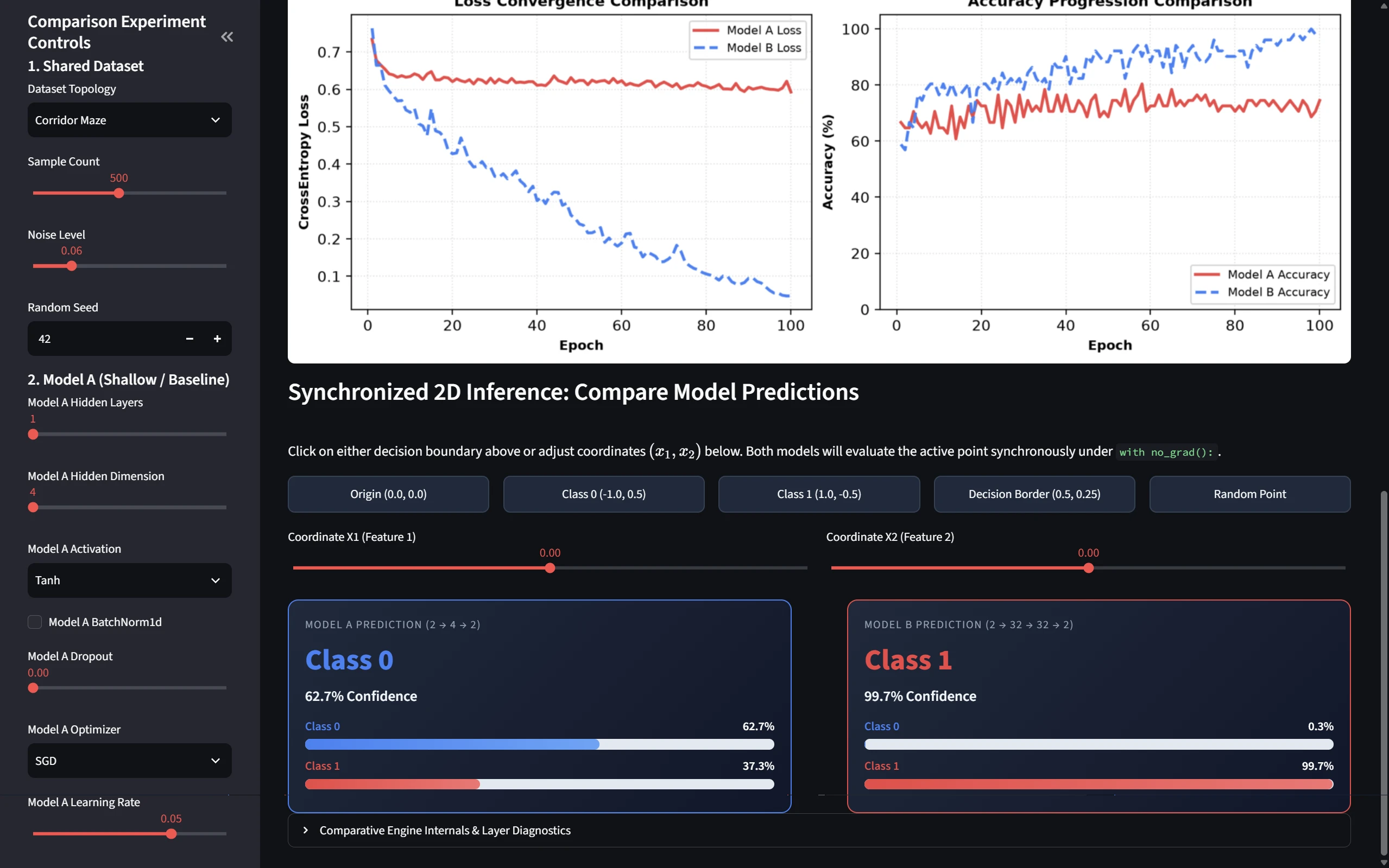
Both models use the same split and mini-batch sequence. The deeper configuration learns the corridor more successfully in this session; architecture, activation, and optimizer all change, so this comparison does not isolate depth alone.
View full-size figureThe supplied session compares a one-layer, four-neuron Tanh model with SGD against a two-layer, 32-neuron ReLU model with AdamW. The shallow configuration’s loss plateaus and its accuracy remains lower, while the larger configuration learns the corridor more successfully.
At the origin, their predictions disagree: Model A selects Class 0 with a 62.7% score; Model B selects Class 1 with a 99.7% score. A shared test point makes the difference tangible, while the maps show how it arises across the wider input space.
The shared data and training batches make the configurations easier to compare. Because architecture, activation, and optimizer all change in this example, it illustrates the behavior of the complete configurations rather than isolating depth alone. This demonstrates experiment design and comparative diagnostics alongside the implementation of multi-model training.
5. Use the learned boundary to guide a rover
The second top-level view turns the classifier into an input for navigation. Class 0 represents free space; the model’s Class 1 score supplies a hazard field. A visitor sets a start and target, adjusts simulation controls, launches a mission, and uses the player to inspect the trajectory and sensor rays step by step.
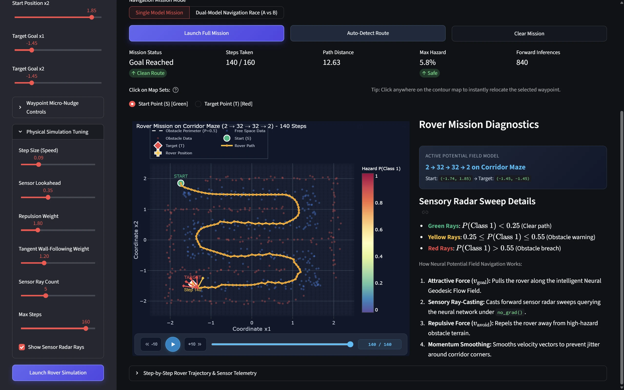
The captured mission reaches the target in 140 steps. A learned hazard field, geodesic guidance, and local sensor queries produce the route; the displayed 5.8% maximum hazard is the model’s score along this simulated run.
View full-size figureThe captured mission follows the corridor from (−1.74, 1.85) toward (−1.45, −1.45) and reports Goal Reached after 140 steps. The recording below shows the rover moving through the route, with its orange trail and forward radar updating along the way.
In this silent recording, the rover advances through the winding corridor, leaving an orange trail as its forward sensor rays update. Playback continues from the first turn to the red target near the lower left. The mission reports Goal Reached after 140 steps.
Download the recordingConnecting prediction to a controller
The controller combines three mechanisms:
- Global guidance: the model evaluates a 45 × 45 grid. An eight-connected Dijkstra distance transform works backward from the goal over hazard-weighted traversal costs; the negative distance gradient supplies a direction through the corridor.
- Local avoidance: five forward rays span −50° to +50° and query the model under
no_grad(). Higher-hazard endpoints contribute a repulsive steering vector. - Smoother movement: the steering blends 80% of the new direction with 20% of the previous direction, then normalizes it before the next step.
The mission view exposes route length, steps, model hazard, and inference counts, making controller behavior inspectable alongside the movement. Its displayed 5.8% maximum hazard is a model score along this particular route; reaching the goal in the demo does not establish safety on arbitrary maps.
I also investigated that distinction in a separate navigation study: 60 trained models and 120 routes, evaluated against a known synthetic obstacle map. A stronger classifier did not guarantee success on every route. Connecting model quality to a downstream outcome demonstrates why classification metrics alone are insufficient for evaluating a navigation system.
6. Draw digits and follow the recognition pipeline
The journey ends in Handwritten Digit Recognition. Visitors draw one or more separated digits, adjust brush width, and use undo, redo, or clear while inspecting the result. The studio presents the recognized sequence, the normalized digit images, top candidates, and a probability breakdown for each digit.
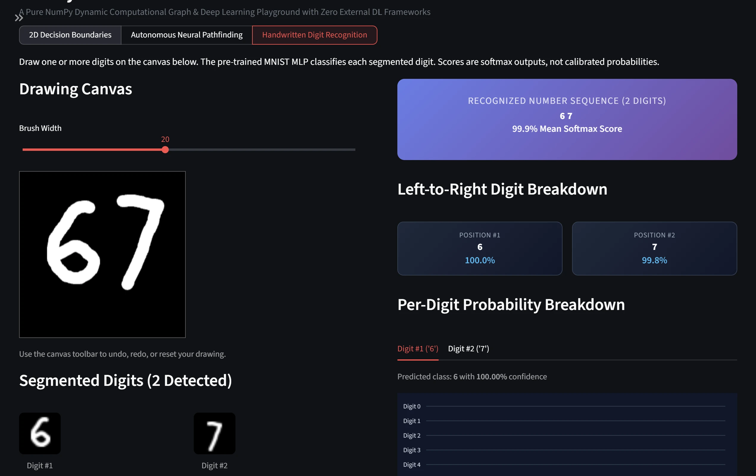
The supplied canvas example is 67. Segmentation and normalization feed each digit into the saved MNIST MLP, which reports 100.0% and 99.8% softmax scores for these two drawings; they are session outputs, not recognition guarantees.
View full-size figureThe supplied example contains 6 and 7. They are segmented left to right and recognized as “67”, with displayed softmax scores of 100.0% and 99.8% for those drawings.
Preparing freehand input for the model
The input pipeline thresholds the drawn strokes, labels connected components, filters small speckles, and merges nearby or overlapping strokes that may belong to one digit. A Python/NumPy component-labeling fallback is available when SciPy is absent. The resulting boxes are ordered left to right.
Each crop is resized to fit within 20 × 20 pixels while preserving its aspect ratio, placed in a 28 × 28 image, shifted toward the center using its pixel mass, and normalized to [0, 1]. These steps bridge the gap between a freely positioned canvas drawing and the input format expected by the MNIST model.
Canvas strokes → component boxes → left-to-right digit crops
  → aspect-preserving resize → 28 × 28 centering → normalization
  → saved model inference → per-digit predictions
Loading and running a model built on the same engine
The studio loads examples/mnist_mlp.ng through my model serializer. Its architecture flattens the image into 784 inputs and applies 784 → 128 → 64 → 10 linear layers with ReLU activations. Inference runs in evaluation mode under no_grad(), then softmax supplies the displayed class scores.
The .ng archive keeps JSON architecture metadata and NumPy parameter arrays together, allowing the loader to reconstruct supported layers and restore their weights. This connects preprocessing, persistence, inference, and presentation in one usable application.
The broader engine also supports convolutional models. I implemented im2col to turn image patches into a matrix multiplication and col2im to accumulate overlapping input-gradient contributions. That trades intermediate memory for vectorized computation; the canvas shown here specifically uses the saved MLP.
NumPyGrad remains a CPU-oriented framework for learning and experimentation. Dynamic graphs make the computation easy to follow, while adding bookkeeping overhead; larger convolution workloads also need care with intermediate memory. Across the studio, the engineering goal is consistent: make a working model usable while keeping its inputs, computations, evaluation, and outputs open to inspection.