Planning for demand before it arrives
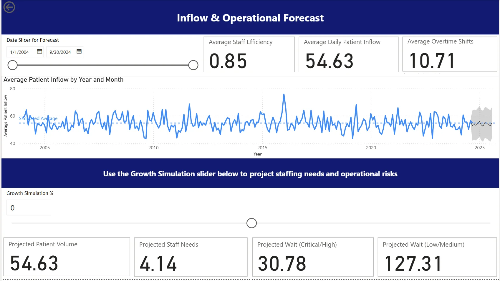
If patient arrivals increase, how much staffing capacity might a hospital need, and which patients could face the greatest waiting-time pressure? I designed this Power BI report around that planning question.
The centrepiece is the Inflow & Operational Forecast dashboard. It brings historical performance, a patient-demand forecast, and an interactive growth scenario into one view. A planner can compare expected demand with a higher-demand scenario and see the implications for staffing and patient waits. I built the full workflow, from preparing three datasets and designing their relationships to writing DAX measures and shaping the dashboard around operational decisions.
Turning a forecast into a capacity decision
I used monthly patient-inflow history spanning 2004–2024 with Power BI’s built-in forecasting, configured for a 12-month horizon and 12-month seasonality. The chart shows the projected trend alongside a shaded forecast range, keeping uncertainty visible when considering future demand.
The Growth Simulation slider adds a second way to plan: test a demand increase and inspect its consequences. It adjusts a simulated inflow reference line and updates projected patient volume, staffing needs, and waits for Critical/High and Low/Medium urgency groups. Putting those outputs together makes the forecast relevant to resource planning: the reader can see what a change in demand means for capacity and patient experience.
The baseline forecast dashboard from the project cover appears again here so its role in the analysis is clear. At zero simulated growth, it establishes the historical KPIs, patient-inflow trend, and forecast range that the growth scenario builds on.
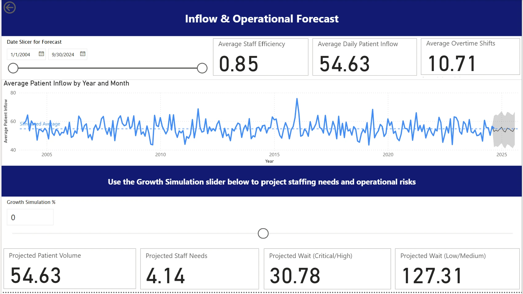
This is the project cover image repeated beside the analysis it introduces. The 0% growth view establishes historical performance and the forecast before a planner tests a higher-demand scenario.
View full-size figureIn the captured 20% demand-growth scenario, the dashboard shows:
| Planning measure | Scenario estimate |
|---|---|
| Patient inflow | 65.56 |
| Staffing need | 4.91 |
| Critical/High urgency wait | 37.56 minutes |
| Low/Medium urgency wait | 165.50 minutes |
The difference between the waiting-time estimates gives a planner a reason to examine how capacity is allocated across urgency groups. This is where the dashboard becomes useful for a discussion about staffing priorities, rather than leaving the reader to interpret an inflow chart alone.
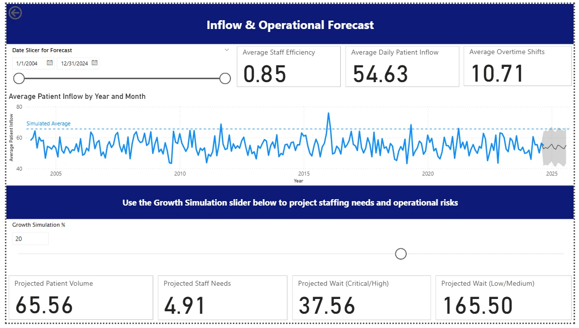
A captured 20% demand-growth scenario brings projected volume, staffing needs, and waits into the same decision view. Historical KPIs remain separate from the scenario estimates.
View full-size figureMaking the interactions meaningful with DAX
I gave the historical KPIs and the growth scenario distinct jobs. Average staff efficiency, daily inflow, and overtime respond to the date slicer, giving the reader a baseline for the selected period. The growth control changes the scenario estimates while keeping those historical measures intact.
For the simulated inflow line, I used CALCULATE with REMOVEFILTERS to calculate an overall historical baseline independently of the chart’s date context. SELECTEDVALUE reads the chosen growth percentage, which scales that baseline. The result is a stable scenario reference across the timeline that can be compared with the forecast range. This required deliberate control of filter context so each interaction answered the intended question.
Building a consistent analytical foundation
The forecast, emergency-wait, and patient-record datasets needed a common time context. I built a star schema with a shared MasterDate dimension, plus a department dimension connecting patient and scheduling data. This supports related operational questions through consistent date and department relationships.
In Power Query, I corrected date types and locale-dependent formats, removed incomplete visit records, deduplicated visit IDs, and standardized hospital names. These choices make the reporting foundation dependable: inconsistent dates or duplicated visits can distort the demand and patient-experience measures a planner relies on.
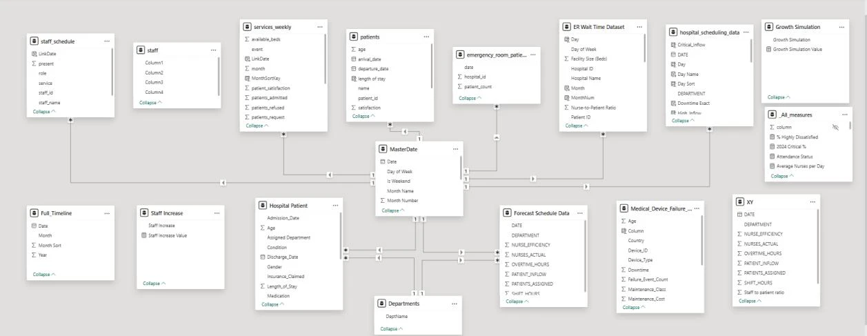
The star schema gives the separate hospital datasets a common date context, with a department dimension linking the patient and scheduling data.
View full-size figureConnecting capacity pressure to patient experience
The supporting patient-experience view uses urgency filters, wait-time bands, and a DAX dissatisfaction measure to locate groups experiencing the longest waits. In the captured data, lower-urgency patients had longer waits and poorer satisfaction. Breaking that down by cohort gives the planning discussion a specific patient group to investigate.
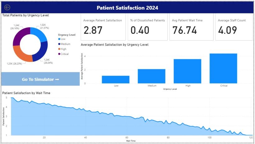
Urgency filters and wait-time bands identify patient groups to investigate when prioritizing capacity. In this view, lower-urgency patients experience longer waits and poorer satisfaction.
View full-size figureA separate staffing simulator lets the reader explore how additional staff could affect waiting time and a corresponding satisfaction indicator. Its wait-time breakdown also helps identify where extra capacity might matter; the captured example highlights time spent waiting for medical professionals.
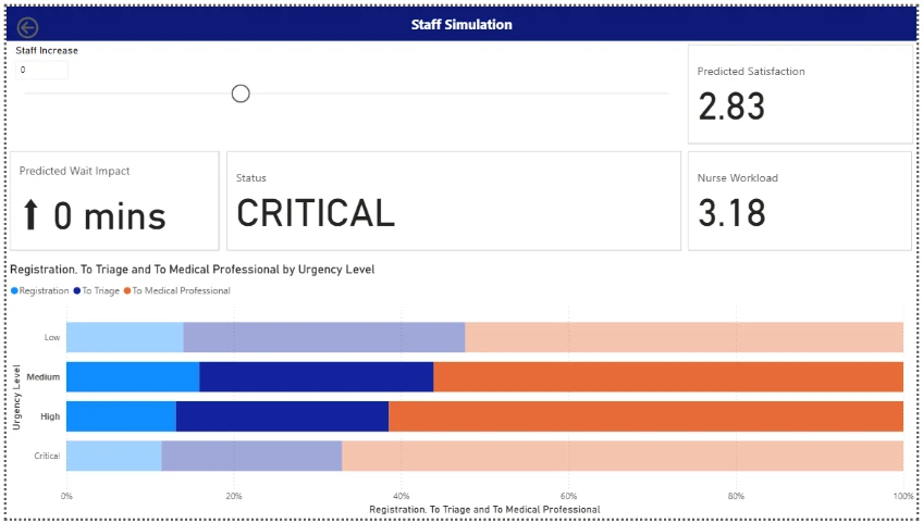
The staffing control tests a proposed capacity change against modeled waits and satisfaction, using an assumed 15% wait reduction per additional staff member.
View full-size figureThe forecast and what-if scenarios serve different purposes: the forecast extrapolates historical patterns, while the scenarios apply chosen assumptions. The staffing simulator assumes a 15% modeled wait reduction per additional staff member. Validating that effect against observed staffing changes would be the next step before using the estimates in an actual staffing plan.